Module 6
Computer Vision
"Computer vision is a complex field, so a lot of research is still needed before all the known - and still unknown - problems can be solved."
About the Module
In this module the main focus is on Computer Vision (CV). The skills and areas of knowledge already learned from the previous chapters should be expanded and stimulate a critical examination of the subject of CV. The "Supervised Learning" module in particular is advantageous for a deeper understanding of the content to come, but it is not compulsory to complete it. Lateral entry is also not a problem and conveys the most important learning objectives.
The aim of this module is to create a basic understanding of how the way of "seeing" differs between humans and computers, which techniques and algorithms enable the detection of objects, but also to create a critical examination and basis for discussion. These goals are achieved primarily through practical "hands-on" and "CS-Unplugged" examples and are completed with a practical example in which the students develop their own machine-learning face-lock program in Scratch. In-depth theoretical knowledge of artificial intelligence and mathematical background knowledge is not necessary.
Objectives
Students will be able to
- name similarities and differences in human and computer-based visual information acquisition
- explain how a computer stores and processes visual information
- know basic algorithms for object recognition and can explain them using simple examples
- apply simple machine learning CV algorithms themselves
- show the limits and possibilities of CV
Agenda
| Time | Content | Material |
|---|---|---|
| 10 min | Introduction | Slides |
| 15 min | Theory - processing of images | Slides |
| 15 min | Theory - Classic CV procedures | Slides |
| 30 min | Theory + Worksheet - Viola Jones | Slides, Worksheet |
| 40 min | Practice - ML Face Recognition with Scratch | Online, Worksheet |
| 10 min | Discussion - possibilities and limits | Slides |
Introduction - What is Computer Vision (CV)?
The introduction to CV is about the students actively dealing with the basic concepts of "seeing" and "object recognition" in a plenary discussion. The presentation slides serve as the basis and guide for this introductory process.
Comparison human - computer
In slides 2-3, the students are introduced to the topic of how people and computers can perceive their environment in a plenary discussion. The important thing here is that the similarities in the basic process between humans and computers are apparent. Various methods (boards, but also various online tools) can be used to collect ideas, etc.
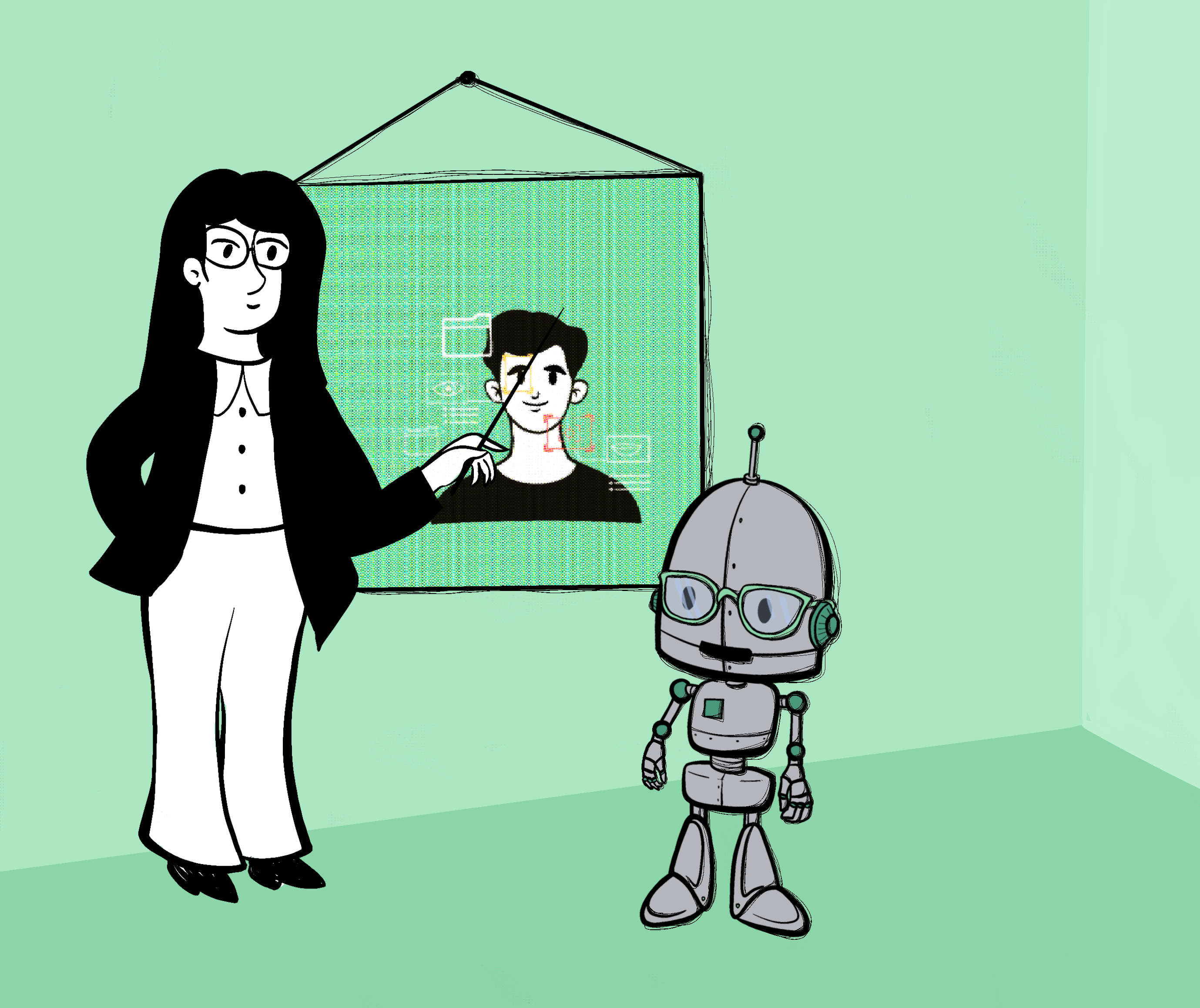
Both humans and computers work according to the principle input - processing - output. We see something with our eyes, process it with our brain and act accordingly. However, before we can work according to this scheme, humans (from infancy onwards) as well as a computer (e.g. supervised learning) must learn certain skills. It is practised iteratively until, for example, you can speak a sentence or recognize an apple as an apple. This initial learning is presented in the first step on slide 5. After the learning process, you can face the challenge and have conversations or distinguish apples from oranges. In the case of the computer, however, we have to provide visual material for the computer to process. That would correspond to the input-step. This is followed by processing by the computer using special computer vision algorithms. The last step is output, in which, for example, the objects in the picture are marked or the mobile phone is unlocked by recognizing the face.
Slide 6 shows some typical CV tasks.
- Classification
- Classification of the object in the photo as a cat
- Classification + Localization
- The cat is also localized in this image and marked with a red rectangle
- Object Detection
- In this example, various objects within the image are classified and also localized
Material
Basics of digital images
In the last section, the topic was fundamentally introduced by means of discussion and examples, which is now to be deepened in the following section with some theoretical basics of digital images. The focus should be on the internal processing and the storage of images.
How are pictures stored in a computer?
In principle, information processing and storage works in a binary way. This means that a computer only knows the states 0 and 1. 0 means no current and 1 means current. Now you have to think about how you can represent vast amounts of image information in 0s and 1s. You have to think outside the box here. To keep things simple, let's look at an image in grayscale. In a grayscale image, different areas of the image appear darker or lighter. The darker a pixel is, the lower its representative numerical value. The value is correspondingly larger for brighter pixels. The number range is from 0 to 255, so 0 is very dark and 255 is very light. If you then convert this decimal number into a binary number (4 => 1000, 3 =>11), you can store it in a computer.
On slide 9 you can see a comparison between human vision and that of a computer. The way in which images are stored in a computer, results in a veritable flood of data. What is exciting, however, is that as soon as you zoom out a little from this mass of numbers, you can even see the content of the image of the turtle stored on the computer with your eyes based on the pixel values only.
What information could already be read from these pixel values? If a light square is adjacent to a dark square, a simple subtraction can reveal a difference in values. Since objects in images usually have some distinctive edges that differ in color from their surroundings, a computer can use simple mathematics, for example, to recognize that it is the edge of a table or the line on a soccer field (more on this later in the Edge Detection chapter).
It works similarly with RGB images, except that much more information is included in the form of numbers. This allows the computer to calculate/save a color and then display it. For the sake of simplicity, we always assume grayscale images in this module.
The only important thing for us at the moment is that we can extract a lot of information from these sets of numbers using special algorithms and various mathematical methods. A simple introduction is to be given by examining together how the flood-fill algorithm works.
Flood Fill
On slide 10, the functioning of the flood fill algorithm is to be worked out by means of a plenary discussion. The students are given time to think about how the algorithm works and to write down the steps. After this phase, possible solutions are discussed and compared in the plenum.
How does the algorithm work? As the name suggests, the image is "flooded" or filled in / painted. Numbers are a good choice here for the ease of illustration. The picture is filled in until another color is found. Depending on which number was drawn, more or less area is painted. Each number has a specific free, unpainted area and can therefore be identified by the computer through mathematical calculations.
Steps: (Example)
- Take two colors (background and font color)
- Place the brush on a starting point
- Paint until the point under the brush has a different color than the background
- When everything is painted, check the level of the brush color
This simple algorithm also has several limitations. For instance, what if the numbers are written improperly and, for example, a zero has an open space and the inner area is also filled out?
Well-known examples of the use of this algorithm would be the legendary Minesweeper game or the area fill function in MS Paint.
Material
Classic CV algorithms
At this point, the students should have a rough idea of how a computer can recognize simple things in digital images. But what if the objects get more complicated, the color differences get blurrier, and the overall complexity increases?
Object recognition often works on the basis of machine and deep learning algorithms, which have been perfected over time. These very complex algorithms can often be replaced by their simpler, classic predecessors. The key word is reducing complexity through abstraction. This is illustrated on slides 14 and 15 using a simple example. Even after removing all image features except for the outline of the elephant, the elephant remains recognizable as an elephant.
Classic edge detection algorithms can be the Sobel or Canny algorithm, for example. These algorithms are very much based on the mathematical foundations of matrix calculation, but clear edges of the objects can already be recognized after partial steps of the algorithm. (Slide 16-24)
Let's think back to the chapter dealing with the storage of images. On slide 16 this internal representation is shown again as an example. It is very easy to see how this robot consists of individual pixels with specific numerical values. Due to the easier handling, the RGB representation of the pixel values is exchanged for that of the grayscale representation, but the principle remains the same. If you look at the numerical values from a certain distance, an approximate shape can already be recognized by the human eye. But how could a computer recognize an "edge" of this object? Right, through mathematical calculations, mainly matrix calculations.
The result of the horizontal edge detection is shown on the following slide 17. The image on the left was created using a Python script and can be made available as an excursus for interested students. The graphic on the right shows the corresponding numerical values after the horizontal edge calculation has been carried out. On slides 18-19 the mathematical technique behind it is explained in more detail. As complicated as these figures look, the algorithm for calculating the value is just as simple. Only basic calculation rules are applied. For example, cell Ab is subtracted from cell Aa and a numerical value is obtained. The higher this numerical value, the greater the color difference between the individual pixels. Ergo, we most likely detected a pixel of an edge. If you do this procedure for all pixel values, you not only get individual values, but whole lines, in this case edges, which can be recognized as such. Now further values of this matrix should be calculated together with the students (the solution can be found in the notes area of the respective slides).
The principle of vertical edge detection works in the same way, so it will not be discussed further. If you have calculated vertical and horizontal edges, you can combine these two results and thus obtain a matrix or an image that now contains all edges. This is visualized again on slides 23, 24 and compared with the original image on slide 25.
In a nutshell, the algorithm consists of the following three steps:
- Calculation of horizontal edges
- Calculation of the vertical edges
- Combination of the two results
Material
Face recognition using the Viola Jones algorithm
Slides 27 to 30 should be discussed with the students as part of a plenary discussion. All the necessary information is on the slides.
Slide 31 shows the first technical basics of the Viola Jones algorithm. An important part of the algorithm is the "sliding window ", which is used to scan the image step by step from left to right and from top to bottom, looking for possible (even multiple) faces and their features. The individual face sections (eyes, nose, mouth, etc.) are recognized with so-called "Haar-like features", which are shown on slide 32.
The main Haar features are:
- edge features
- line features
- four-rectangle features
These features and the sliding window do not have a fixed size but are dynamically adjusted as needed. This procedure is shown again on slide 33 and a video is also linked on slide 34, which summarizes and visualizes the process of the Viola Jones algorithm.
The Viola Jones algorithm has some limitations: It can only detect frontal faces, which could be problematic in certain scenarios and use cases and entail the need to use further computer vision methods. It is also important to emphasize that while Viola Jones can detect faces, it cannot distinguish different faces.
Next (slides 35 - 36) is the hands-on example of the Viola Jones algorithm. The materials required and the explanation of the task can be found in the worksheet file and on the slides. In addition, there is the possibility for interested or advanced students to try out the Viola Jones algorithm using a Python script (the task and sample solution can be found on slide 37).
Material
Machine Learning in CV
On slide 39 you will find a short summary. Computer Vision (CV) and Machine Learning (ML) are two areas of AI. Computer vision deals with the computer-based processing of visual information, which can be further improved by machine learning approaches (e.g. recognition of movements, sequences of objects in real time, ...). Since machine learning - especially supervised learning - has already been taken up and discussed in another module, we next focus on "hands-on" examples in which ML and CV are combined.
The students are supposed to program a virtual smartphone using a previously created machine learning model. The necessary documents and explanations can be found in the corresponding worksheet file.
Material
Opportunities and Limitations
Computer vision is a complex field, so a lot of research is still needed before all the known - and still unknown - problems can be solved. In addition, we have also seen that even algorithms as simple as the Viola Jones algorithm have been used practically everywhere for decades. At the end of this module, any questions, comments, etc. from the students should be addressed and an exchange should take place. On slide 42 there are some suggested questions that can be used as a starting point for a dynamic discussion.
If there is still time at this point, slide 43 can be discussed further. Here, an image of a traffic light classified by a computer is changed by simply changing pixels in such a way that the CV algorithm is no longer able to classify the traffic light correctly. Further information regarding the reliability of CV algorithms can be found on the homepage linked on slide 43 in the notes section.